A continuous probability distribution is a representation of a variable that can take a continuous range of values.

The continuous uniform distribution is a family of symmetric probability distributions in which all intervals of the same length are equally probable.
The exponential distribution is a family of continuous probability distributions that describe the time between events in a Poisson process.
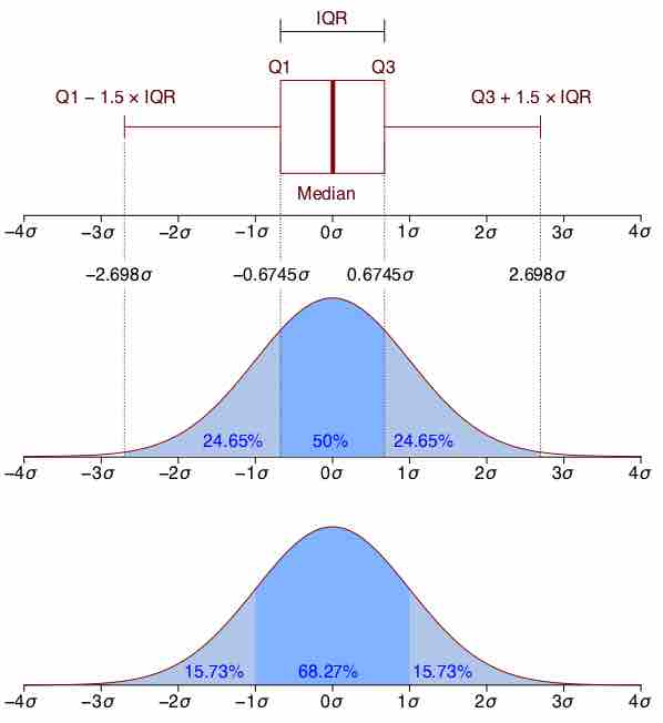
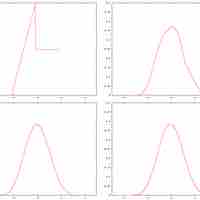
The normal distribution is symmetric with scores more concentrated in the middle than in the tails.
The graph of a normal distribution is a bell curve.
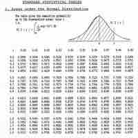
The standard normal distribution is a normal distribution with a mean of 0 and a standard deviation of 1.

To calculate the probability that a variable is within a range in the normal distribution, we have to find the area under the normal curve.
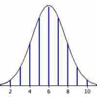
The process of using the normal curve to estimate the shape of the binomial distribution is known as normal approximation.
The scope of the normal approximation is dependent upon our sample size, becoming more accurate as the sample size grows.
In this atom, we provide an example on how to compute a normal approximation for a binomial distribution.
In order to consider a normal distribution or normal approximation, a standard scale or standard units is necessary.

Systematic, or biased, errors are errors which consistently yield results either higher or lower than the correct measurement.

Random, or chance, errors are errors that are a combination of results both higher and lower than the desired measurement.
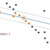
In statistics, an outlier is an observation that is numerically distant from the rest of the data.
A probability histogram is a graph that shows the probability of each outcome on the

Many different types of distributions can be approximated by the normal curve.
Many distributions in real life can be approximated using normal distribution.