Introduction

Once you have entered information into a spreadsheet, you may want to format it. Formatting your spreadsheet can not only improve the look and feel of your spreadsheet, but it also can make it easier to use. In a previous lesson, we discussed many manual formatting options such as bold and italics. In this lesson, you'll learn how to format as a table to take advantage of the tools and predefined table styles available in Excel 2010.

Formatting tables

Just like regular formatting, tables can help to organize your content and make it easier for you locate the information you need. To use tables effectively, you'll need to know how to format information as a table, modify tables, and apply table styles .

Optional: You can download this example for extra practice.

To format information as a table:

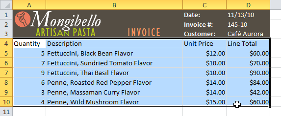
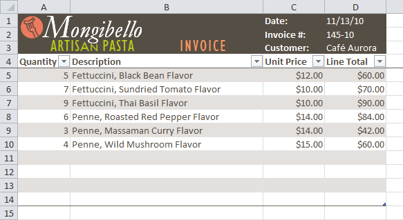
1. Select the cells you want to format as a table. In this example, an invoice, we'll format the cells containing the column headers and order details.
   Selecting cells to format as a table
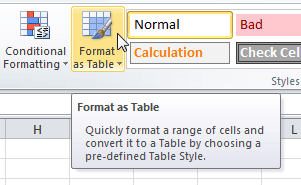
2. Click the Format as Table command in the Styles group on the Home tab.
   Format as Table command
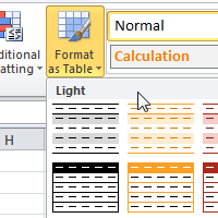
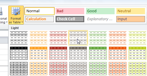
3. A list of predefined table styles will appear. Click a table style to select it.
   Selecting a table style
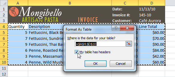
4. A dialog box will appear, confirming the range of cells you have selected for your table. The cells will appear selected in the spreadsheet, and the range will appear in the dialog box.
5. If necessary, change the range by selecting a new range of cells directly on your spreadsheet.
6. If your table has headers, check the box next to My table has headers .
   Creating a table
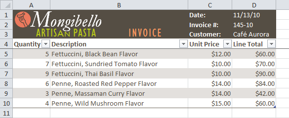
7. Click OK . The data will be formatted as a table in the style you chose.
   Data formatted as a table

Tables include filtering by default. You can filter your data at any time using the drop-down arrows in the header. To learn more, review our Filtering Data lesson.

To convert a table back into normal cells, click the Convert to Range command in the Tools group. The filters and Design tab will then disappear, but the cells will retain their data and formatting.

Modifying tables

To add rows or columns:

1. Select any cell in your table. The Design tab will appear on the Ribbon.
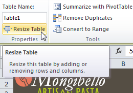
2. From the Design tab, click the Resize Table command.
   Resize Table command
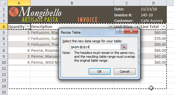
3. Directly on your spreadsheet, select the new range of cells you want your table to cover. You must select your original table cells as well.
   Selecting a new range of cells
4. Click OK . The new rows and/or columns will be added to your table.
   After adding new rows

To change the table style:

1. Select any cell in your table. The Design tab will appear.
2. Locate the Table Styles group. Click the More drop-down arrow to see all of the table styles.
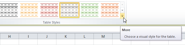   The More drop-down arrow
3. Hover the mouse over the various styles to see a live preview.
4. Select the desired style. The table style will appear in your worksheet.
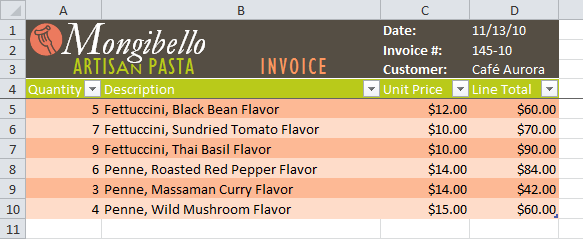   After changing the table style

To change table style options:

When using an Excel table, you can turn various options on or off to change its appearance. There are six options: Header Row , Total Row , Banded Rows , First Column , Last Column , and Banded Columns .

1. Select any cell in your table. The Design tab will appear.
2. From the Design tab, check or uncheck the desired options in the Table Style Options group.
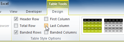   Table style options

Depending on the table style you're using, certain table style options may have a different effect. You may need to experiment to get the exact look you want.

Challenge!

1. Open an existing Excel 2010 workbook . If you want, you can use this example .
2. Format a range of cells as a table . If you are using the example, format the column headers (Quantity, Description, etc.) and the order details.
3. Add a row or a column.
4. Change the table style options . If you are using the example, add a total row.
5. Change the table style several times. Take note of how the table options may appear different depending on the style you use.