How to use Excel's VLOOKUP function

Many of our learners have told us they want to learn how to use Excel's VLOOKUP function. VLOOKUP is an extremely useful tool, and learning how to use it is easier than you think!

Before you start, you should understand the basics of functions. Check out our Functions lesson from our Excel Formulas tutorial (or select a specific version of Excel ). VLOOKUP works the same in all versions of Excel, and it even works in other spreadsheet applications like Google Sheets. You can download the example if you'd like to work along with this article.

What exactly is VLOOKUP?

Basically, VLOOKUP lets you search for specific information in your spreadsheet. For example, if you have a list of products with prices, you could search for the price of a specific item.

We're going to use VLOOKUP to find the price of the Photo frame . You can probably already see that the price is $9.99, but that's because this is a simple example. Once you learn how to use VLOOKUP, you'll be able to use it with larger, more complex spreadsheets, and that's when it will become truly useful.

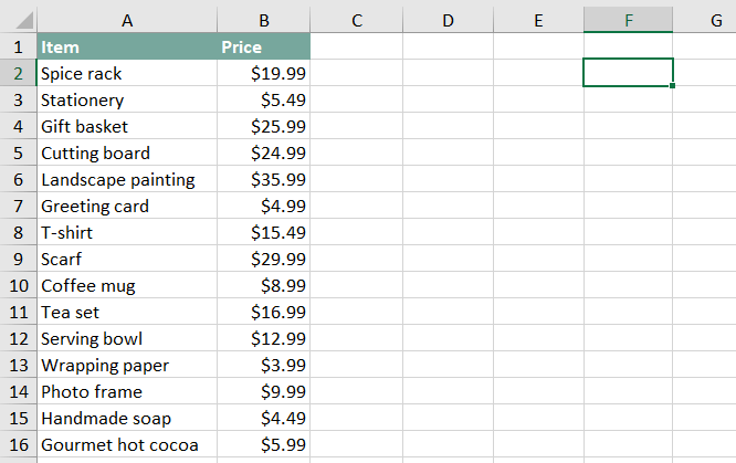
We'll add our formula to cell F2 , but you can add it to any blank cell. As with any formula, you'll start with an equals sign (=). Then type the formula name. Our arguments will need to be in parentheses, so type an open parenthesis. So far, it should look like this:

=VLOOKUP(

Adding the arguments

Now, we'll add our arguments. The arguments will tell VLOOKUP what to search for and where to search.

The first argument is the name of the item you're searching for, which in this case is Photo frame . Because the argument is text, we'll need to put it in double quotes:

=VLOOKUP("Photo frame"

The second argument is the cell range that contains the data . In this example, our data is in A2:B16. As with any function, you'll need to use a comma to separate each argument:

=VLOOKUP("Photo frame", A2:B16

It's important to know that VLOOKUP will always search the first column in this range. In this example, it will search column A for "Photo frame". The value that it returns (in this case, the price) will always need to be to the right of that column.

The third argument is the column index number . It's simpler than it sounds: The first column in the range is 1, the second column is 2, etc. In this case, we are trying to find the price of the item , and the prices are contained in the second column . This means our third argument will be 2 :

=VLOOKUP("Photo frame", A2:B16, 2

The fourth argument tells VLOOKUP whether to look for approximate matches , and it can be either TRUE or FALSE. If it is TRUE, it will look for approximate matches. Generally, this is only useful if the first column has numerical values that have been sorted. Because we're only looking for exact matches, the fourth argument should be FALSE . This is our last argument, so go ahead and close the parentheses:

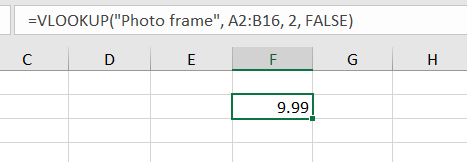
=VLOOKUP("Photo frame", A2:B16, 2, FALSE)

That's it! When you press Enter, it should give you the answer, which is 9.99 .

How it works

Let's take a look at how this formula works. It first searches vertically down the first column (VLOOKUP is short for vertical lookup ). When it finds "Photo frame", it moves to the second column to find the price.

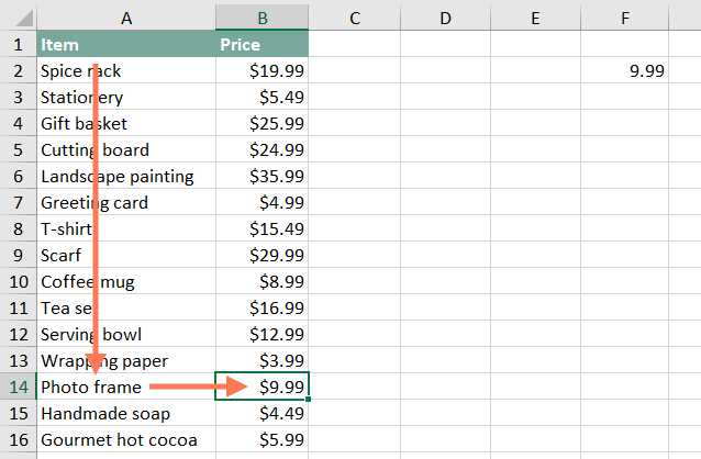
As we mentioned earlier, the price needs to be to the right of the item name. VLOOKUP cannot look to the left of the column that it's searching.

If we want to find the price of a different item, we can just change the first argument:

=VLOOKUP("T-shirt", A2:B16, 2, FALSE)

or:

=VLOOKUP("Gift basket", A2:B16, 2, FALSE)

It would be very tedious to edit your VLOOKUP formula whenever you want to find the price of a different item. In the next example, we'll show how to avoid this by using a cell reference.

Another example

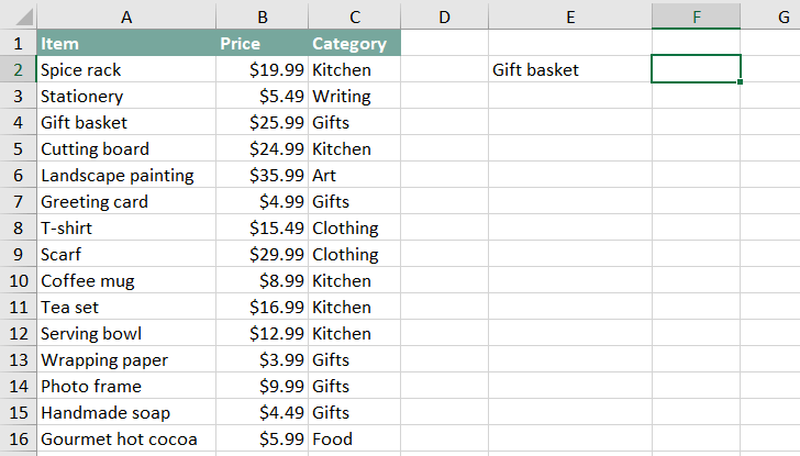
Are you ready for a slightly more advanced example? We're going to make a couple of changes to the spreadsheet to make it more realistic.

In the previous example, we typed the item name directly into the VLOOKUP formula. But in the real world, you'll usually use a cell reference instead. In this example, we'll type the item name in cell E2 , and our VLOOKUP formula can then use a cell reference to find information about that product. Then, we can simply type a new item name into E2 to find any product we want.

We've also added a third column that has the category for each item. This will give us the option of finding the price or category. Here's what the spreadsheet looks like so far:

Our formula will be similar to the previous example, but we'll need to change the first three arguments . Let's start by changing the first argument to a cell reference (make sure to remove the quotation marks):

=VLOOKUP(E2, A2:B16, 2, FALSE)

To find the category, we'll need to change the second and third arguments . First, we'll change the range to A2:C16 so it includes the third column. Next, we'll change the column index number to 3 because our categories are in the third column:

=VLOOKUP(E2, A2:C16, 3, FALSE)

When you press Enter, you'll see that the Gift basket is in the Gifts category.

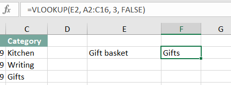
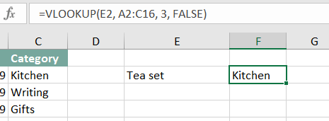
If we want to find the category of a different item, we can simply change the item name in cell E2 :

Try this!

If you'd like more practice, see if you can find the following:

• The price of the coffee mug
• The category of the landscape painting
• The price of the serving bowl
• The category of the scarf

Now that you know the basics of VLOOKUP, you can use it in many different situations. For example, if you have a contact list you could search for someone's name to find his or her phone number. If your contact list has columns for the email address or company name, you could search for those by simply changing the second and third arguments, as we did in our example.

To get even more practice with VLOOKUP, you can check out the Invoice series in our Excel Formulas tutorial. It covers tips for avoiding common problems and using data validation to use VLOOKUP with a drop-down list!